Application of Spatial Priors in the Maximum Likelihood Classification of Tropical Dry Forest Classes

by J. Ronald Eastman and Florencia Sangermano

Introduction

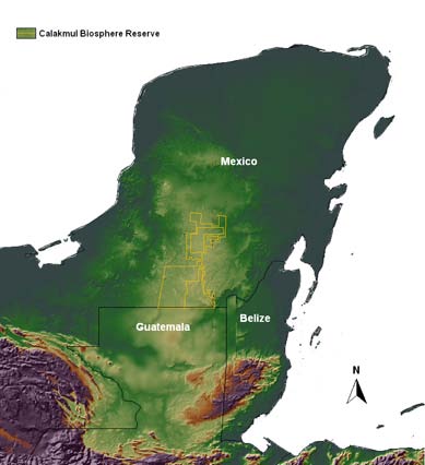
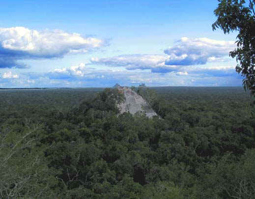
Over the past four years, the Southern Yucatan Peninsula Region (SYPR) Project has been engaged in an effort to develop a detailed mapping of tropical forest classes in the region of the Calakmul Biosphere Reserve (see Turner et al., 2004). The Calakmul Biosphere Reserve (Figure 1) is the largest continuous forest area region in Mexico and an important component of the Meso-American Biological Corridor. It is also a significant cultural resource with an extraordinary range of Mayan sites including Calakmul, Becán and Hormiguero (Figure 2). Unfortunately, the region has been experiencing continuing pressure from development at its margins. A central goal of the SYPR Project has been to understand, model and monitor the intricate relationship between humans and the environment in the general region of this important environmental reserve, and to ultimately gauge the implications of that relationship for biodiversity. An important component of this activity has been the mapping of land cover classes – largely natural seasonally dry tropical forest classes – over time.

The Southern Yucatan Peninsula Region is a karstic region in which subtle variations in seasonal precipitation can lead to substantial differences in vegetation condition. Since wet season imagery is predominantly covered by clouds, archival imagery tends to come from the dry season. Figure 3 illustrates the strongly variable extent of deciduousness as evident in Landsat TM and ETM+ imagery.

However, even in cases where there is adequate moisture to retain leaf cover, substantial variability can still exist and forest cover types can look different from one year to the next (Figure 4). Development of a comparable land cover classification over time is thus very challenging.

General Logic

To develop a comparable time series of classified Landsat imagery, a novel approach was employed, using the Bayesian soft classification module (BAYCLASS) in conjunction with IDRISI’s unique ability to allow spatially explicit prior probabilities in its Maximum Likelihood classification module (MAXLIKE)1.

The field work and the majority of the classification effort were directed to an exceptionally clear and advantageously timed image from March of 2000. Our logic was to use this resulting classification as an input (only for the forest classes) to the classification of the other images. In this manner, knowledge of forest classes in 2000 was used to influence the classification of other years. This is based on the assumption that the forest classes are stable and that any change from forest to non-forest would be associated with a dramatic change in spectral response pattern.

1 The potential of doing this was explored in detail by Strahler (1980). However, this is the only implemention that we are aware of in a commercially distributed software package.

Creating the Prior Probability Images

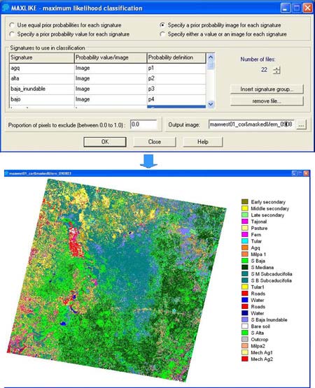
After the training sites were developed on the image (March 2000), we ran the BAYCLASS module (Figure 5). BAYCLASS produces a set of images (one for each class) expressing the posterior probabilities of belonging to each class based on the standard Maximum Likelihood discriminant function:

 

 

where
c = a land cover class
x = a vector of reflectances for a pixel
p(ci) = prior probability of a class
p(x|ci) = conditional probability derived from the training data (see below)
p(ci|x) = posterior probability of belonging to a class

and

 

 

where
i = mean vector of class i
Vi = variance/covariance matrix of class i
n = number of classes

For the next step, only the forest class images were used.

We adjusted the posterior probabilities to account for error since we could not assume the classification was perfectly accurate. As this preceded our accuracy assessment, we assumed an accuracy level of 85%. The formula used to accommodate this was:

 

 

 

where
p(cf) = prior probability of a forest class
p(cf|x) = posterior probability of belonging to a forest class
n = total number of classes

Since the posterior probabilities are images in this case, we used the Macro Modeler in IDRISI Kilimanjaro to apply this formula to each of the forest class posterior probability images, yielding a set of spatially explicit prior probability images (i.e., the prior probability varies from one pixel to the next). To create prior probability images for the non-forest classes, we used the following formula:

 

 

 

where
p(cnf) = prior probability of a non-forest class
p(cnf|x) = posterior probability of belonging to a non-forest class
n = total number of classes
k = number of forest classes

Again Macro Modeler was used to apply this formula to the non-forest posterior probability images. The result was a set of prior probability images that are spatially explicit, but which are identical between non-forest classes.

Incorporating Ancillary Information — Modifying the Priors

A number of land cover classes (both forest and non-forest) were found to have topographic preferences. For example, Figure 6 shows the difference in relative frequency of bracken fern (an invasive plant species) for varying slope gradients. (The graph was created by subtracting the relative frequency with which varying slope gradients occur in the image from the relative frequency with which bracken fern is found in the same slope gradient bins. Negative values indicate a lower than chance probability and positive values indicate a higher than chance probability. As can be seen, bracken fern has a decided preference for slopes greater than 2.5% in this region.)

Incorporating such information into the prior probability images of any class is fairly simple and requires the following steps:

1. Use the ASSIGN module to assign the residual relative frequencies (residual probabilities) to the appropriate bins (slope gradient bins in this example).
2. Add the result to the prior probability image for the class concerned.
3. Divide the result by (n-1) and subtract it from the prior probability images for all other classes.

Classification Using the Spatial Priors

Once the prior probability images were developed (and modified as necessary) for all classes, the MAXLIKE module was run using the “spatial priors” option (Figure 7).

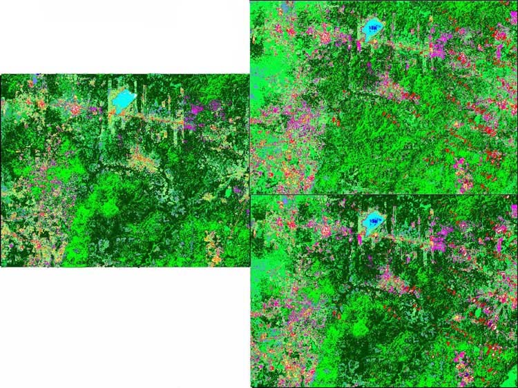
Figure 8 shows a detailed comparison of the results for 2001 with and without this knowledge along with the classification for 2000 which was the basis for the priors. Our experience with the use of spatial priors is that it can make a substantial and positive difference in difficult classification tasks. A quantitative assessment of this difference will be reported in a forthcoming article (Eastman et al., forthcoming).

 

References

Eastman, J.R., Sangermano, F., and Dickson, R.P., (forthcoming). Derivation and Application of Spatially-Explicit Prior Probabilities for Land Cover Classification.

Lawrence, D., Vester, H., Pérez-Salicrup, D., Eastman, J.R., Turner II, B. L., and Geoghegan, J. 2003. Integrated Analysis of Ecosystem Interactions with Land-Use Change: The Southern Yucatán Peninsular Region. In Ecosystem Interactions with Land Use Change, G. Asner and R. DeFries, eds., Geophysical Monograph Series 153: 277-292 Washington, D.C.: American Geophysical Union.

Strahler, A.H.1980. The use of prior probabilities in maximum likelihood classification of remotely sensed data. Remote Sensing of Environment 10: 135-163.

B. L. Turner II, J. Geoghegan, and D. Foster, eds. 2004. Integrated Land-Change Science and Tropical Deforestation in the Southern Yucatán: Final Frontiers. Oxford Geographical and Environmental Studies. Clarendon Press of Oxford University Press.